How to User Slicers in Microsoft Excel 2010

Overview
Slicers are the new feature in Excel 2010 which has got everyone talking. Essentially Slicers are a user-friendly filtering system which makes PivotTables & PivotCharts easier to work with and now brings a high level of dashboard capability to Excel.




First Create Your PivotTables
The first step in using Slicers is to create your PivotTables & PivotCharts:

1. Select the Insert tab on the Ribbon then click the PivotTable button and choose PivotChart.
2. Next select the data range and choose to create the PivotTable and PivotChart on a new worksheet (once we have created a dashboard we can hide the PivotTable tabs)
3. Now choose the required fields in the Field List to create your PivotTable & Chart.
4. Finally cut and past the PivotChart into a new worksheet. This will form the basis of our ‘Dashboard’.
5. Repeat the above process as necessary to create further PivotCharts and place them on the dashboard.

Each of the PivotCharts on the dashboard can be individually filtered directly using the Field Buttons. However, the slicers we create next will take over this function and provide a higher level of interactivity between PivotCharts. We can therefore remove the Field Buttons, here’s how:

1. Click inside the PivotChart and the PivotChart Tools group will appear on the Ribbon.
2. Next select the Analyze tab and click the Field Buttons menu.
3. Choose Hide All to remove the Field Buttons on the PivotChart.

Creating the Slicer
The next step is to create slicers to add real functionality to the dashboard:

1. First click inside a PivotChart and then select the Insert Slicer button menu. Choose Insert Slicer from drop-down the menu.
2. You will be presented with a dialogue box containing a list of PivotTable fields.
3. Choose appropriate fields to wish to filter then click OK.

How to Use Slicers
The slicer will be created as a box with a number of buttons which enabling filtering. Clicking an individual button will change the PivotChart accordingly. Multiple selections can be made by holding down the CTRL key. The filter can be removed by either clicking the funnel icon or alternatively dragging across all the buttons to select them all.

Enhancing Slicer Functionality
A major advantage of using Slicers is the ability to filter multiple PivotCharts simultaneously, creating true dashboard functionality. Here’s how to link PivotCharts together:

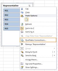
1. First select a Slicer and right-click in the header area (where the Slicer title appears), then choose PivotTable Connections from the menu. Alternatively you can select the Options tab on the Ribbon and choose PivotTable Connections.
2. Next select from available PivotTables those that you wish to connect to the Slicer.
3. Finally click OK to complete the process.

Creating a Dashboard
We now have the basis for a full dashboard system which enables simultaneous filtering of multiple data fields. Simply set up all your PivotCharts on one spreadsheet tab and create Slicers with multiple connections as necessary. Group your Slicers with the PivotCharts and you will have a user-friendly data filtering system. You may find it advantageous to colour code your charts and slicers to match, so that you can filter data more easily:

1. To change you PivotTable colour, first select the Design tab in the PivotChart tools group.
2. You can now select from a range of chart colours in the PivotChart styles gallery.
3. To change Slicer colours, first click a slicer then select the Options / Slicer Tools tab on the Ribbon.
4. A corresponding colour can now be selected from the Slicer Styles gallery.

Summary
Slicers represent a powerful new filtering tool in Excel 2010 which appears set to transform the way that we use PivotTables and PivotCharts.